leaderbot Documentation#
leaderbot is a python package that provides a leaderboard for chatbots based on Chatbot Arena project.
Install#
Install with pip:
pip install leaderbot
Alternatively, clone the source code and install with
cd source_dir
pip install .
Quick Usage#
The package provides several statistical ranking models (see
API reference for details). In the example below, we use
leaderbot.models.Davidson class to create a model. However, working
with other models is similar.
Create and Train a Model#
>>> from leaderbot.data import load
>>> from leaderbot.models import Davidson

>>> # Create a model
>>> data = load()
>>> model = Davidson(data)

>>> # Train the model
>>> model.train()
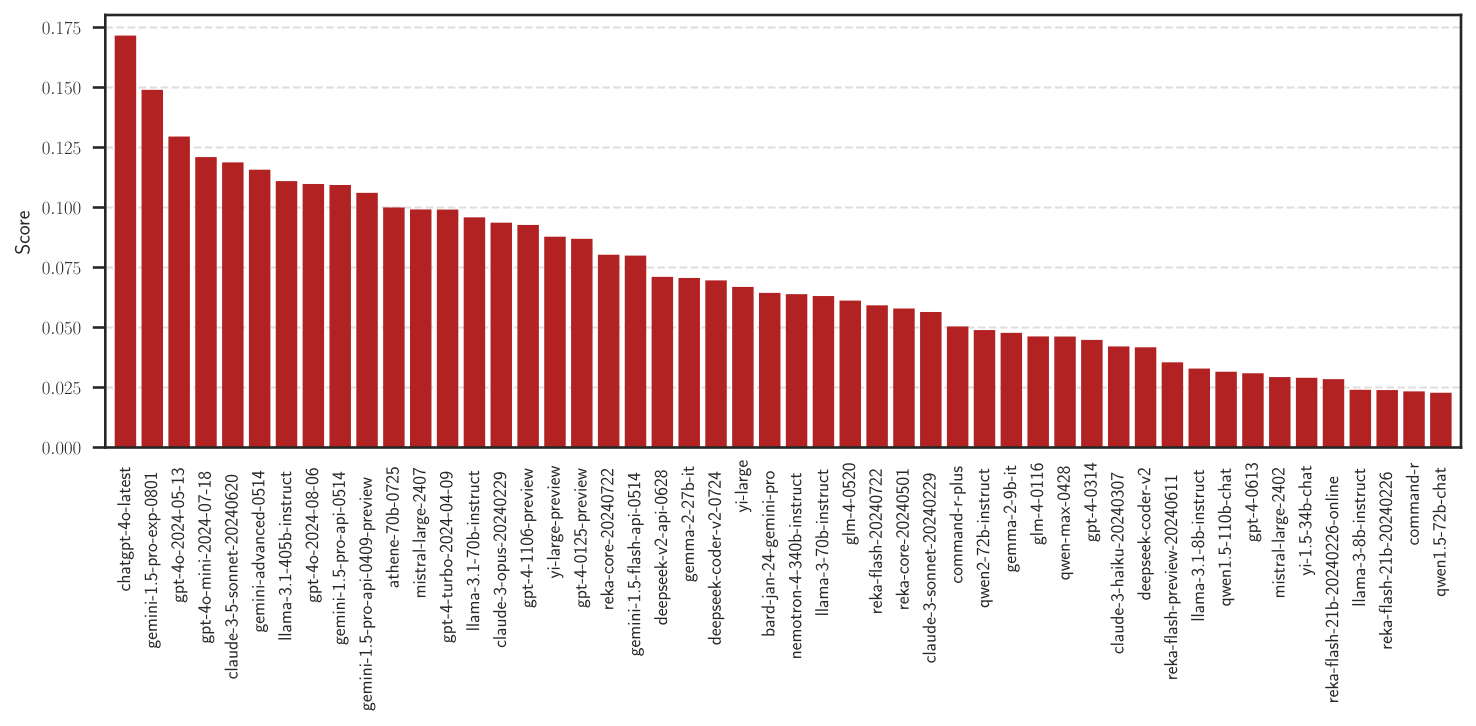
Leaderboard Table#
To print leaderboard table of the chatbot agents, use
leaderbot.models.Davidson.leaderboard() function:
>>> # Leaderboard table
>>> model.leaderboard(max_rank=30)
The above code prints the table below:
+---------------------------+--------+--------+---------------+---------------+
|                           |        |    num |   observed    |   predicted   |
| rnk  agent                |  score |  match | win loss  tie | win loss  tie |
+---------------------------+--------+--------+---------------+---------------+
|   1. chatgpt-4o-latest    | +0.172 |  11798 | 53%  23%  24% | 53%  23%  24% |
|   2. gemini-1.5-pro-ex... | +0.149 |  16700 | 51%  26%  23% | 51%  26%  23% |
|   3. gpt-4o-2024-05-13    | +0.130 |  66560 | 51%  26%  23% | 51%  26%  23% |
|   4. gpt-4o-mini-2024-... | +0.121 |  15929 | 46%  29%  25% | 47%  29%  24% |
|   5. claude-3-5-sonnet... | +0.119 |  40587 | 47%  31%  22% | 47%  31%  22% |
|   6. gemini-advanced-0514 | +0.116 |  44319 | 49%  29%  22% | 49%  29%  22% |
|   7. llama-3.1-405b-in... | +0.111 |  15680 | 44%  32%  24% | 44%  32%  23% |
|   8. gpt-4o-2024-08-06    | +0.110 |   7796 | 43%  32%  25% | 43%  32%  25% |
|   9. gemini-1.5-pro-ap... | +0.109 |  57941 | 47%  31%  22% | 47%  31%  22% |
|  10. gemini-1.5-pro-ap... | +0.106 |  48381 | 52%  28%  20% | 52%  28%  20% |
|  11. athene-70b-0725      | +0.100 |   9125 | 43%  35%  22% | 43%  35%  22% |
|  12. mistral-large-2407   | +0.099 |   9309 | 41%  35%  25% | 41%  34%  25% |
|  13. gpt-4-turbo-2024-... | +0.099 |  73106 | 47%  29%  24% | 47%  29%  24% |
|  14. llama-3.1-70b-ins... | +0.096 |  10946 | 41%  36%  22% | 41%  37%  22% |
|  15. claude-3-opus-202... | +0.094 | 134831 | 49%  29%  21% | 49%  29%  21% |
|  16. gpt-4-1106-preview   | +0.093 |  81545 | 53%  25%  22% | 53%  25%  22% |
|  17. yi-large-preview     | +0.088 |  42947 | 46%  32%  22% | 45%  31%  23% |
|  18. gpt-4-0125-preview   | +0.087 |  74890 | 49%  28%  23% | 49%  28%  22% |
|  19. reka-core-20240722   | +0.080 |   5518 | 39%  39%  22% | 39%  39%  22% |
|  20. gemini-1.5-flash-... | +0.080 |  45312 | 43%  35%  22% | 43%  35%  22% |
+---------------------------+--------+--------+---------------+---------------+
Score Plot#
The scores versus rank can be plotted by
leaderbot.models.Davidson.plot_scores() function:
>>> model.plot_scores(max_rank=50)
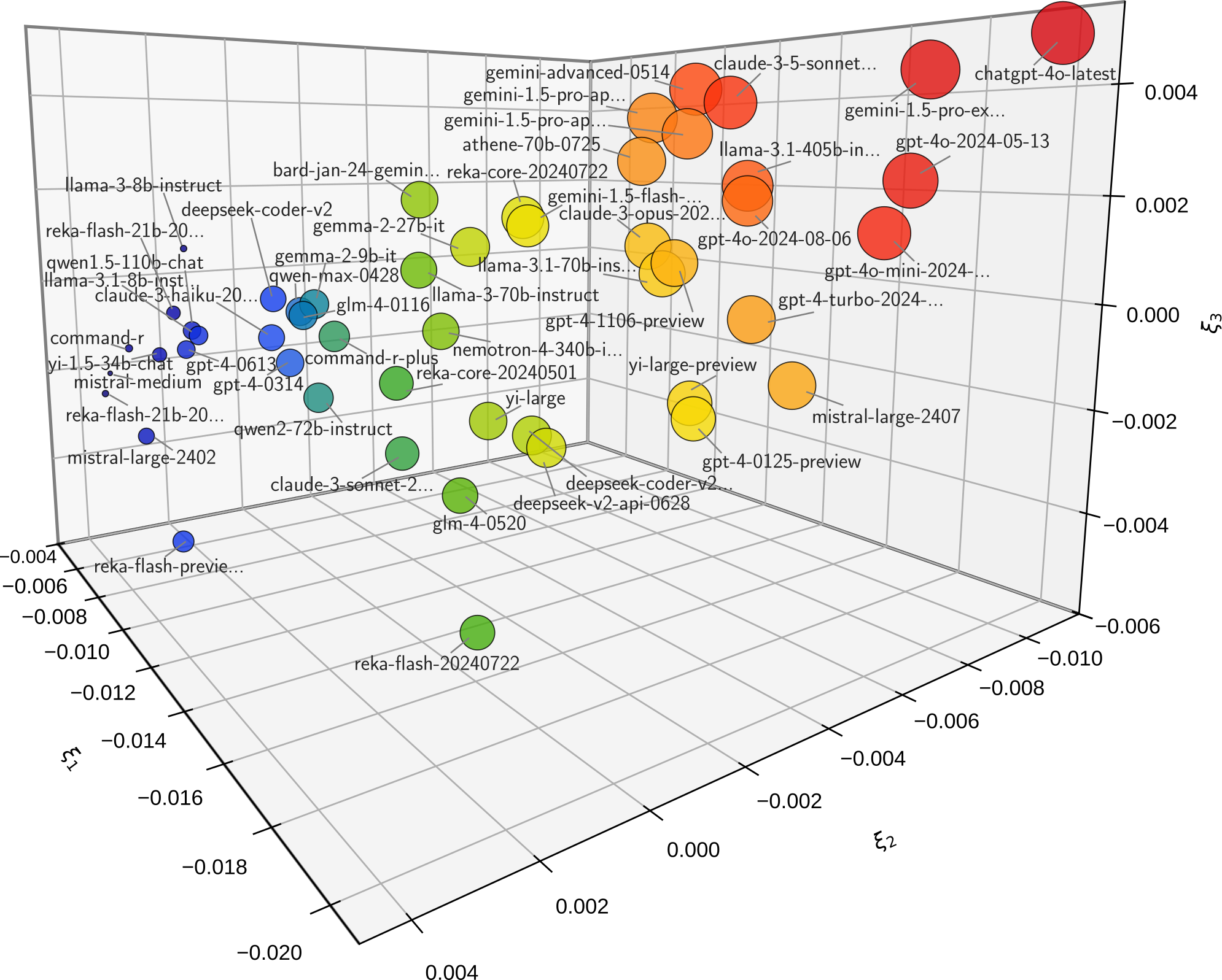
Visualize Correlation#
The correlation of the chatbot performances can be visualized with
leaderbot.models.Davidson.map_distance() using various methods. Here is
an example with the Kernel PCA method:
>>> # Plot kernel PCA
>>> model.map_distance(max_rank=50, method='kpca', dim='3d')
The above code produces plot below demonstrating the Kernel PCA projection on three principal axes:
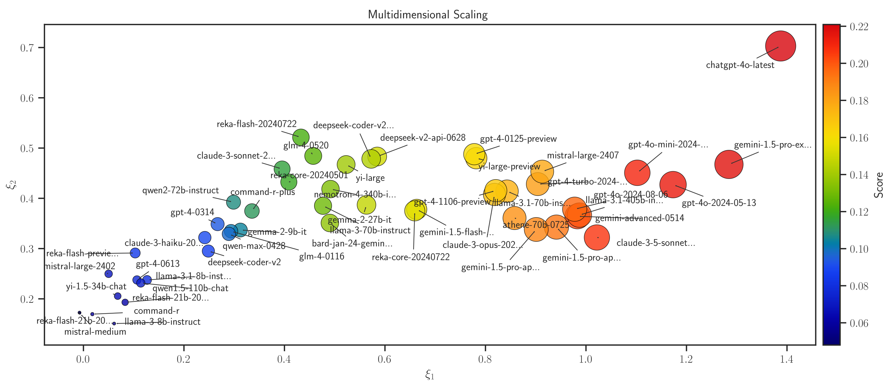
Similarly, the correlation distance between competitors can be visualized using multi-dimensional scaling(MDS)
>>> # Plot MDS
>>> model.map_distance(max_rank=50, method='mds', dim='2d')
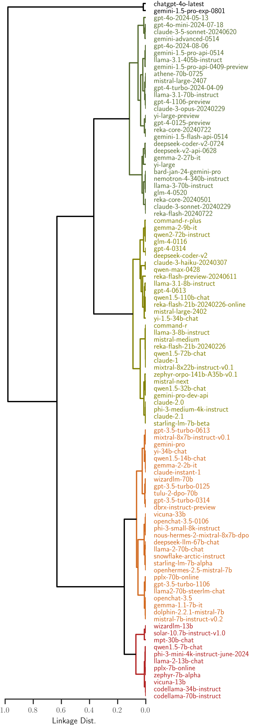
Hierarchical Clustering#
The function leaderbot.models.Davidson.cluster() performs hierarchical
clustering of the chatbots based on the score and correlation distances:
>>> # Plot hierarchical cluster
>>> model.cluster(max_rank=100)
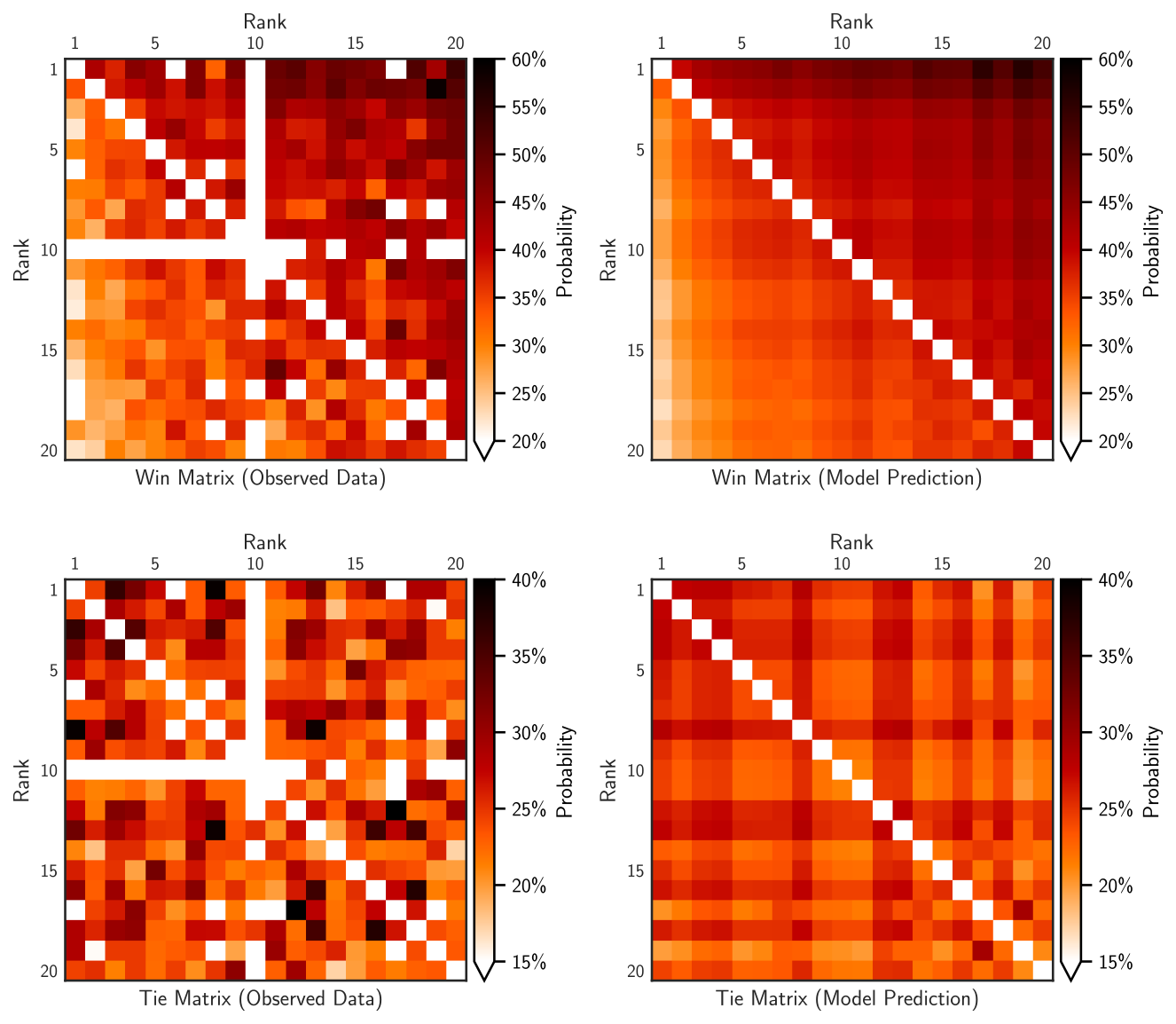
Match Matrices#
The match matrices of the counts or densities of wins and ties can be
visualized with leaderbot.models.Davidson.match_matrix() function:
>>> # Match matrix for probability density of win and tie
>>> model.match_matrix(max_rank=20, density=True)
Marginal Outcomes#
The marginal probabilities (or frequencies) of win, loss, and tie outcomes can
be plotted with leaderbot.models.Davidson.marginal_outcomes() function:
>>> # Plot marginal probabilities
>>> model.marginal_outcomes(max_rank=100)
Make Inference and Prediction#
Once a model is trained, you can make inference on the probabilities of win,
loss, or tie for a pair of agents using leaderbot.models.Davidson.infer()
and leaderbot.models.Davidson.predict() methods:
>>> # Create a list of three matches using pairs of indices of agents
>>> matches = list(zip((0, 1, 2), (1, 2, 0)))

>>> # Make inference
>>> prob = model.infer(matches)

>>> # Make prediction
>>> pred = model.predict(matches)
Model Evaluation#
Performance of multiple models can be compared as follows. First, create a list of models and train them.
>>> import leaderbot as lb
>>> from leaderbot.models import BradleyTerry as BT
>>> from leaderbot.models import RaoKupper as RK
>>> from leaderbot.models import Davidson as DV

>>> # Obtain data
>>> data = lb.data.load()

>>> # Create a list of models to compare
>>> models = [
...    BT(data, k_cov=None),
...    BT(data, k_cov=0),
...    BT(data, k_cov=1),
...    RK(data, k_cov=None, k_tie=0),
...    RK(data, k_cov=0, k_tie=0),
...    RK(data, k_cov=1, k_tie=1),
...    DV(data, k_cov=None, k_tie=0),
...    DV(data, k_cov=0, k_tie=0),
...    DV(data, k_cov=0, k_tie=1)
... ]

>>> # Train models
>>> for model in models:
...    model.train()
Model Selection#
Model selection can be performed with
leaderbot.evaluate.model_selection():
>>> # Evaluate models
>>> metrics = lb.evaluate.model_selection(models, report=True)
The above model evaluation performs the analysis via various metric including the negative log-likelihood (NLL), cross entropy loss (CEL), Akaike information criterion (AIC), and Bayesian information criterion (BIC), and prints a report these metrics the following table:
+----+--------------+---------+--------+--------------------------------+---------+---------+
|    |              |         |        |               CEL              |         |         |
| id | model        | # param |    NLL |    all     win    loss     tie |     AIC |     BIC |
+----+--------------+---------+--------+--------------------------------+---------+---------+
|  1 | BradleyTerry |     129 | 0.6554 | 0.6553  0.3177  0.3376     inf |   256.7 |  1049.7 |
|  2 | BradleyTerry |     258 | 0.6552 | 0.6551  0.3180  0.3371     inf |   514.7 |  2100.8 |
|  3 | BradleyTerry |     387 | 0.6551 | 0.6550  0.3178  0.3372     inf |   772.7 |  3151.8 |
|  4 | RaoKupper    |     130 | 1.0095 | 1.0095  0.3405  0.3462  0.3227 |   258.0 |  1057.2 |
|  5 | RaoKupper    |     259 | 1.0092 | 1.0092  0.3408  0.3457  0.3228 |   516.0 |  2108.2 |
|  6 | RaoKupper    |     516 | 1.0102 | 1.0102  0.3403  0.3453  0.3245 |  1030.0 |  4202.1 |
|  7 | Davidson     |     130 | 1.0100 | 1.0100  0.3409  0.3461  0.3231 |   258.0 |  1057.2 |
|  8 | Davidson     |     259 | 1.0098 | 1.0098  0.3411  0.3455  0.3231 |   516.0 |  2108.2 |
|  9 | Davidson     |     387 | 1.0075 | 1.0075  0.3416  0.3461  0.3197 |   772.0 |  3151.1 |
+----+--------------+---------+--------+--------------------------------+---------+---------+
Goodness of Fit#
The goodness of fit test can be performed with
leaderbot.evaluate.goodness_of_fit():
>>> # Evaluate models
>>> metrics = lb.evaluate.goodness_of_fit(models, report=True)
The above model evaluation performs the analysis of the goodness of fit using mean absolute error (MAE), KL divergence (KLD), Jensen-Shannon divergence (JSD), and prints the following summary table:
+----+--------------+----------------------------+------+------+
|    |              |             MAE            |      |      |
| id | model        |   win   loss    tie    all | KLD% | JSD% |
+----+--------------+----------------------------+------+------+
|  1 | BradleyTerry |  18.5   18.5  -----   18.5 | 1.49 | 0.44 |
|  2 | BradleyTerry |  15.3   15.3  -----   15.3 | 1.42 | 0.42 |
|  3 | BradleyTerry |  12.9   12.9  -----   12.9 | 1.40 | 0.42 |
|  4 | RaoKupper    |  27.5   31.1   45.4   34.7 | 3.32 | 0.92 |
|  5 | RaoKupper    |  26.2   29.6   45.7   33.8 | 3.23 | 0.90 |
|  6 | RaoKupper    |  25.1   27.8   42.8   31.9 | 3.28 | 0.87 |
|  7 | Davidson     |  28.6   32.2   49.0   36.6 | 3.41 | 0.94 |
|  8 | Davidson     |  27.5   30.8   49.3   35.9 | 3.32 | 0.92 |
|  9 | Davidson     |  24.1   25.0   35.7   28.2 | 2.93 | 0.81 |
+----+--------------+----------------------------+------+------+
Generalization#
To evaluate generalization, we first train the models on 90% of the data (training set) and test against the remaining 10% (test set).
>>> import leaderbot as lb
>>> from leaderbot.models import BradleyTerry as BT
>>> from leaderbot.models import RaoKupper as RK
>>> from leaderbot.models import Davidson as DV

>>> # Obtain data
>>> data = lb.data.load()

>>> # Split data to training and test data
>>> training_data, test_data = lb.data.split(data, test_ratio=0.2)

>>> # Create a list of models to compare
>>> models = [
...    BT(training_data, k_cov=None),
...    BT(training_data, k_cov=0),
...    BT(training_data, k_cov=1),
...    RK(training_data, k_cov=None, k_tie=0),
...    RK(training_data, k_cov=0, k_tie=0),
...    RK(training_data, k_cov=1, k_tie=1),
...    DV(training_data, k_cov=None, k_tie=0),
...    DV(training_data, k_cov=0, k_tie=0),
...    DV(training_data, k_cov=0, k_tie=1)
... ]

>>> # Train models
>>> for model in models:
...    model.train()
We can then evaluate generalization on the test data using
leaderbot.evaluate.generalization() function:
>>> # Evaluate models
>>> metrics = lb.evaluate.generalization(models, test_data, report=True)
The above model evaluation computes prediction error via mean absolute error (MAE), KL divergence (KLD), Jensen-Shannon divergence (JSD), and prints the following summary table:
+----+--------------+----------------------------+------+------+
|    |              |             MAE            |      |      |
| id | model        |   win   loss    tie    all | KLD% | JSD% |
+----+--------------+----------------------------+------+------+
|  1 | BradleyTerry |  18.5   18.5  -----   18.5 | 1.49 | 0.44 |
|  2 | BradleyTerry |  15.3   15.3  -----   15.3 | 1.42 | 0.42 |
|  3 | BradleyTerry |  12.9   12.9  -----   12.9 | 1.40 | 0.42 |
|  4 | RaoKupper    |  27.5   31.1   45.4   34.7 | 3.32 | 0.92 |
|  5 | RaoKupper    |  26.2   29.6   45.7   33.8 | 3.23 | 0.90 |
|  6 | RaoKupper    |  25.1   27.8   42.8   31.9 | 3.28 | 0.87 |
|  7 | Davidson     |  28.6   32.2   49.0   36.6 | 3.41 | 0.94 |
|  8 | Davidson     |  27.5   30.8   49.3   35.9 | 3.32 | 0.92 |
|  9 | Davidson     |  24.1   25.0   35.7   28.2 | 2.93 | 0.81 |
+----+--------------+----------------------------+------+------+
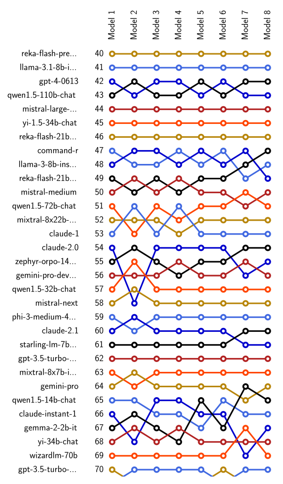
Comparing Ranking of Models#
Ranking of various models can be compared using
leaderbot.evaluate.compare_ranks() function:
>>> import leaderbot as lb
>>> from leaderbot.models import BradleyTerry as BT
>>> from leaderbot.models import RaoKupper as RK
>>> from leaderbot.models import Davidson as DV

>>> # Load data
>>> data = lb.data.load()

>>> # Create a list of models to compare
>>> models = [
...     BT(data, k_cov=0),
...     BT(data, k_cov=3),
...     RK(data, k_cov=0, k_tie=0),
...     RK(data, k_cov=0, k_tie=1),
...     RK(data, k_cov=0, k_tie=3),
...     DV(data, k_cov=0, k_tie=0),
...     DV(data, k_cov=0, k_tie=1),
...     DV(data, k_cov=0, k_tie=3)
... ]

>>> # Train the models
>>> for model in models: model.train()

>>> # Compare ranking of the models
>>> lb.evaluate.compare_ranks(models, rank_range=[40, 70])
The above code produces plot below.
API Reference#
Check the list of functions, classes, and modules of leaderbot with their usage, options, and examples.
Test#
You may test the package with tox:
cd source_dir
tox
Alternatively, test with pytest:
cd source_dir
pytest
How to Contribute#
We welcome contributions via GitHub’s pull request. Developers should review our Contributing Guidelines before submitting their code. If you do not feel comfortable modifying the code, we also welcome feature requests and bug reports.
