leaderbot.models.Davidson.map_distance#
- Davidson.map_distance(ax=None, cmap=None, max_rank=None, method='kpca', dim='3d', sign=None, bg_color='none', fg_color='black', save=False, latex=False)#
Visualize distance between agents using manifold learning projection.
- Parameters:
- axmpl_toolkits.mplot3d.axes3d.Axes3D, default=None
Axis object for plotting. If None, a 3D axis is created.
- cmapmatplotlib.colors.LinearSegmentedColormap, default=None
Colormap for the plot. If None, a default colormap is used.
- max_rankint, default=None
The maximum number of agents to be displayed. If None, all agents in the input dataset will be ranked and shown.
- method{
'kpca','mds'} Method of visualization:
'kpca': Kernel-PCA'mds': Multi-Dimensional Scaling
- dimtuple or {
'2d','3d'} Dimension of visualization. If a tuple is given, the specific axes indices in the tuple is plotted. For example,
(2, 0)plots principal axes \((x_2, x_0)\).- signtuple, default=None
A tuple consisting -1 and 1, representing the sign each axes. For example,
sign=(1, -1)together withdim=(0, 2)plots the principal axes \((x_0, -x_2)\). If None, all signs are assumed to be positive.- bg_colorstr or tuple, default=’none’
Color of the background canvas. The default value of
'none'means transparent.- fg_colorstr or tuple, default=’black’
Color of the axes and text.
- savebool, default=False
If True, the plot will be saved. This argument is effective only if
plotis True.- latexbool, default=False
If True, the plot is rendered with LaTeX engine, assuming the
latexexecutable is available on thePATH. Enabling this option will slow the plot generation.
- Raises:
- RuntimeError
If the model is not trained before calling this method.
Examples
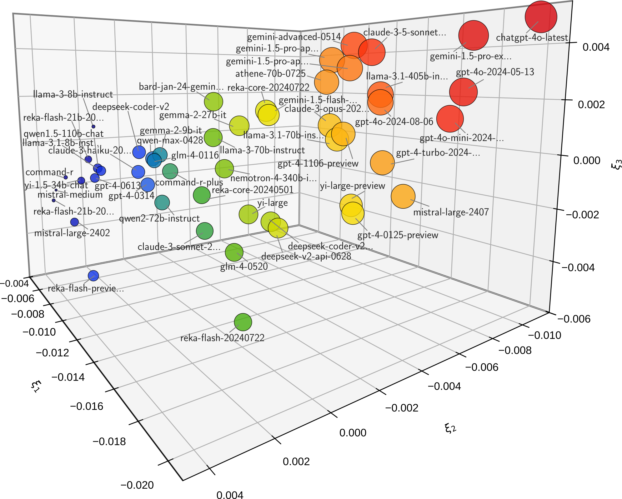
The following example uses Kernel-PCA method projected on 3-dimensional space:
>>> from leaderbot.data import load
>>> from leaderbot.models import Davidson

>>> # Create a model
>>> data = load()
>>> model = Davidson(data)

>>> # Train the model
>>> model.train()

>>> # Plot kernel PCA
>>> model.map_distance(max_rank=50)
The above code produces plot below.
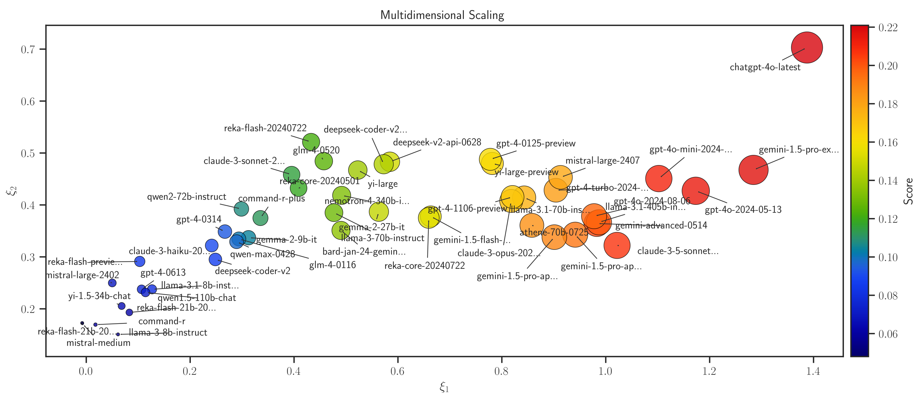
The example below uses MDS method projected in 2-dimensional space:
>>> # Plot MDS
>>> model.map_distance(max_rank=50, method='mds', dim='2d')